Sampling riparian vegetation

There are endless variations to the ways we survey vegetation – and there needs to be. A particular vegetation survey will need to meet specific requirements of accuracy, cost efficiency, relevance and purpose. For example, within the same study site, survey methods used for a study on species richness will be very different from a study on how life form cover changes over time.

This need to tailor vegetation surveys towards the specific study results in difficulties when comparing data from different sources. It is inappropriate to compare say, species richness data, between two sites (or even the same site) if the data were collected using different methods – unless you have quantified the bias in each method. This is because of the different biases and uncertainties associated with each survey method. Many of these biases are evaluated and compared in the literature but I won’t go into that any further here.

Vegetation attributes of different vegetation types are influenced by different things, for example, riparian vegetation is greatly influenced by water levels and flows whereas alpine vegetation is greatly influenced by temperatures and snow cover. Survey methods may need to accommodate these effects.

Riparian vegetation

Location along a water course and distance from the water’s edge impact vegetation attributes. This is due to the response of vegetation to available water,  the destructive effects of water flows and also other factors linked to water, e.g. livestock spend time near water to drink.  Surveys of riparian vegetation should at least acknowledge these gradients, as we do for any other environmental gradient such as altitude.

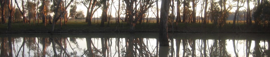
Riparian vegetation in northern Victoria

Distance from the stream

The surveys for my PhD recorded vegetation at point quadrats along transects running away from a creek edge. These data estimated the cover of a range of vegetation life forms (e.g. native shrubs and exotic annual herbs) and ground covers (e.g. litter and bare ground) across sites along this gradient of near to far from the creek edge. The data showed that many of these covers vary along this gradient. You can read the paper when it comes out to get the full details but in general some things do change a lot and others don’t.

It is then interesting to know what sorts of things may influence vegetation along this gradient. A large suite of potential drivers are candidates for this such as, rainfall, vegetation composition, livestock grazing, tree cover, etc.

An example for both of the above points is presented below for bare ground. Bare ground in my study was highest very close to the creek where low level erosion and water flows prevent plants from establishing. This effect was increased by the presence of grazing. The animals spend a lot of time near the water to drink and for shade and in the process eat and trample the vegetation close to the creek. Bare ground tended to gradually increase further from the creek, which is likely due to the proximity to the adjacent agricultural land. Let me know if you want to know more. I have done these types of assessment for all of the life forms.

Bare ground percent cover with increasing distance from creek. Each point represents data across all sites at that distance from the creek. Grey dots are data from sites where grazing was present and back dots from sites without grazing. Solid lines are a segmented linear regression of these data, dashed lines occur at the change point of these lines. Red fitted lines are loess models of the data.

Increased plant suppression and soil erosion on stream bank due to livestock

Distance along the stream

The additional gradient along the length of the stream varies in stream width (wider downstream) and the concentration of sediment, propagules and nutrients that accumulate along its path. This accumulation generally results in an increase in vegetation cover across a range of life forms. An example of this is shown in the figure below for native shrub cover. The relationship is quite poor (R-squared 0.10) as this relationship does not take into account any other site factors such as grazing, management, size, etc that will influence shrub cover.

Native shrub cover versus distance upstream of the creek confluence with the Murray River. Each point indicates a site. The line is a linear model of this relationship (R-squared = 0.10).

Summary

Riparian vegetation studies should attempt to account for the natural variation along these two riparian specific gradients as part of their survey design. Each different riparian system will have its own effects on vegetation and extrapolation of relationships to other systems should be done with caution.

This is just a taste of some of the work I have been doing on this particular issue. Keep your eyes peeled for more information. If you simply can’t wait until then, feel free to contact me.